An Implementation of the Marching Cubes[1] Algorithm
By Ben Anderson
Abstract:
The Marching cubes algorithm can be described as follows:
Given an object, a test to determine whether an arbitrary point is
within the object, and bounds within which the object exists:
Divide the space within the bounds into an arbitrary number of
cubes. Test the corners of every cube for whether they are inside
the object. For every cube where some corners are inside and some
corners are outside the object, the surface must pass through that
cube, intersecting the edges of the cube in between corners of opposite
classification. Draw a surface within each cube connecting these
intersections. You have your object.
Full Text:
Once we have masked images of every slice of the object we are to
reconstruct (ie, a black and white image where black is inside and
white is outside the object), we can go about reconstructing the
original surface. One way of doing this is to use the Marching
Cubes algorithm[2].
In 2D:
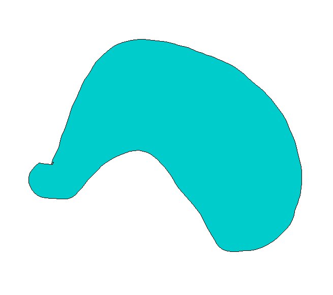
To understand how the Marching Cubes algorithm works, let's take a 2D
case and what might be called the "Marching Squares" algorithm.
Here's our object:
Now, let's divide it into squares:
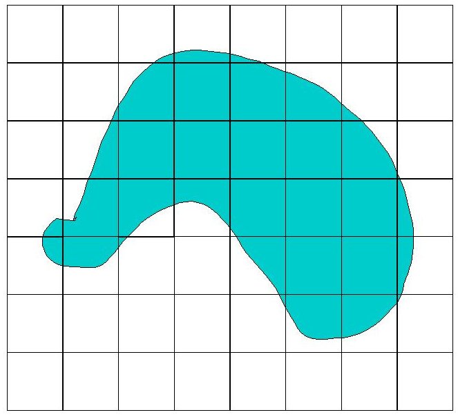
We can tell by looking at it which vertices are in, and which are
outside of the object, so let's label them, red for inside, blue for
out:

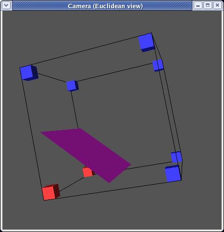
Now we know that somewhere on each edge between an inside corner and an
outside one the original surface must intersect our squares (purple
dots):

Within each square, let's connect the purple dots. Now we have an
approximation of the original surface (the purple lines):

In 3D:
Implementing the algorithm in 3D works much the same as it did in
2D. For slice data like the Visible Human Male dataset, you stack
the slices in 3D, knowing each slice is 1mm or 3 pixels appart.
In order to be able to test the vertices of each cube, you must choose
your cube size to align with the slices, either using 1mm cubes (or
rectangles 1mm high and 1/3rd of a mm thick since pixels are only 1/3rd
of a mm wide), or some multiple of 1mm cubes (ie 2mm or 3 mm) so that
each horizontal side of your cubes falls on the plane of a slice.
You then can test each vertex by going to the masked slices
corresponding to each cube's top and bottom z values. You now
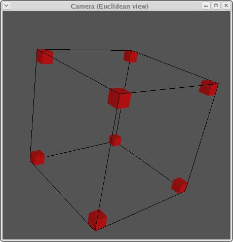
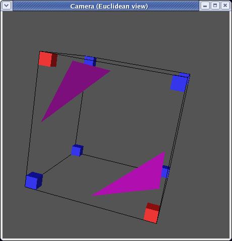
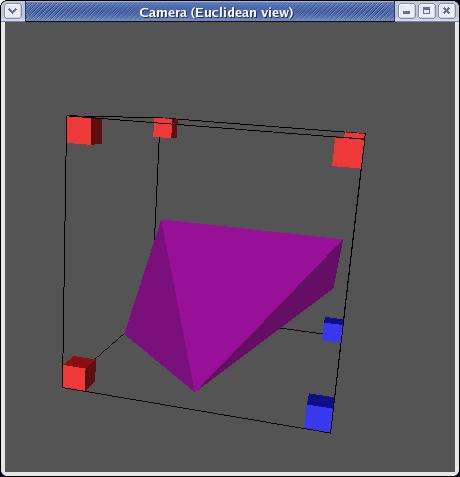
have a bunch of cubes with labeled corners. For each cube, you
know the surface intersects the cube along the edges in between corners
of opposing classifications. Each cube should look something like
this:

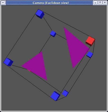
In 2D to approximate the surface we simply had to draw lines between
each purple dot. In 3D this would give us a strange line drawing
like this:

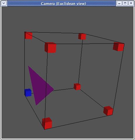
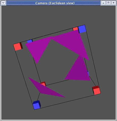
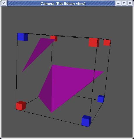
Which doesn't look very much like a piece of a circle. Instead,
what we want to do is triangulate the cube where filled triangles will
represent the surface passing through the cube. Something like
this:

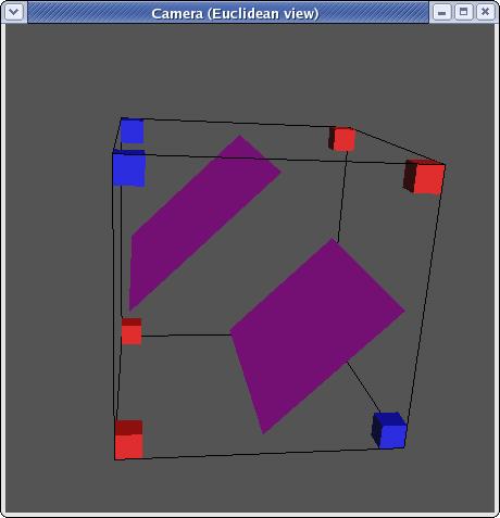
However, you'll note that this isn't as easy as drawing a line
connecting all the purple dots in a square. For one thing, a
triangle connects 3 dots, and for another, it's hard to tell which
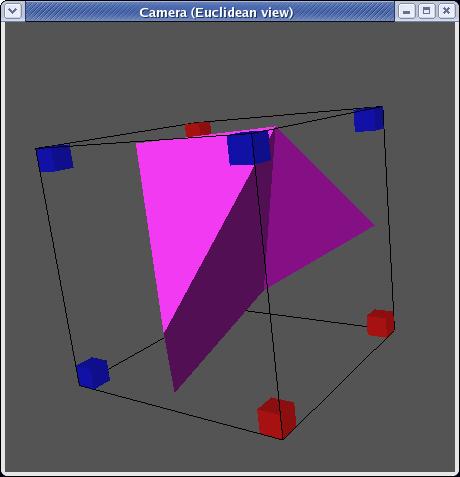
three dots to connect in which triangle. If you just randomly
connected dots in a triangle, you might get something like:

Which really doesn't look any good. The other issue is that since
you're going to be doing this to a lot of cubes, you probably want
whatever solution you find to be fast. And what is really
fast? A lookup table. Consider a cube. Each corner
can be either inside or outside the object. There are eight
corners. That means you're working with 28, or 256
different possibilities for what a cube might look like, which is
definitely feasible. Triangulating each of those possibilities
might be a pain, but luckily, given identical triangulations for cubes
whose vertex classification is opposite of eachother, rotations and
mirroring, there are in fact only 14 unique triangulations:


Each triangulation contains zero to four triangles and can be stored as
a list of triangles where each triangle is a list of 3 numbers which
are indexes to the edges on which each triangles vertices lie. for an
example, here's some ASCII art taken from the code labeling each edge
and each corner with an index:
//
v7_______e6_____________v6
//
/|
/|
//
/
|
/ |
//
e7/
|
e5/ |
//
/___|______e4_________/ |
//
v4|
|
|v5 |e10
//
|
|
| |
//
|
|e11
|e9 |
//
e8|
|
| |
//
| |_________________|___|
//
| / v3
e2 | /v2
//
|
/
| /
//
|
/e3
| /e1
//
|/_____________________|/
//
v0
e0 v1
As you can see, the triangle in the second example might be defined as
[e3,e2,e11]. A cube can be looked up in the table by taking the
classification of each vertex and converting it to 0's and 1's and then
forming a binary number. Again, using the same cube as an
example, v3 is inside the shape and every other vertex is out.
This results in a binary number of 00010000 or 23 or 8, so
the entry for 8 in the lookup table might be:
8: [e1,e2,e11]
In the actual code, it doesn't look quite like that, but you get the
idea.
And so, in order to compute the triangulation for the entire image, you
do this for every cube, offset the triangulations to their appropriate
locations in the space and voila!

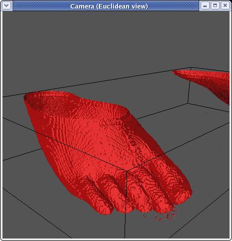
As you can tell, this is a blocky rendering of a foot. You were
probably hoping for somthing better. Well, luckily, this is only
rendered using 1/3rd of the slices, (fairly big cubes). To
overcome this, the first thing you might think of is to make the cubes
smaller resulting in a more accurate rendering of a foot:

Well, that's better, but as you can tell, it's still fairly
blocky. Well, we can do better. To understand how, let's go
back to 2D.
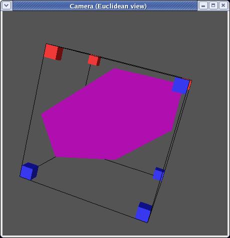
Here's our approximation in 2D from earlier:
Now, without even using smaller cubes, we can come up with a much
better approximation of this surface, and one that's much smoother (the
surface right now is made up of facets meeting at 45°
angles). How can we do that? Like this:

The only difference here is that the purple dots have been moved.
Instead of placing the purple dots midway between the red and the blue
ones, they have been moved to meet up with the actual intersection of
the surface with the edges in question. This results in a more
accurate representation of the surface, as well as a smoother one using
the same number of cubes as before. Let's see what that looks
like in 3D:
Now, that is smoother, and you can almost make out the toenail ont he
big toe, but if you're saying to yourself, "That's still pretty
blocky," you'd be right.
The main problem is that while in 2D we can compute exact intersections
for every edge of our shape, given only slice data, in 3D, we cannot do
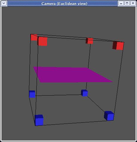
this. Take this picture for example:
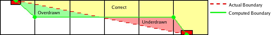
This is a side view of a row of cubes. The top line is a slice,
as is the bottom. The problem is that while we can compute exact
intersections on a given slice, in between, we have no idea where the
object lies. While the actual surface is represented by the
dotted red line, in between layers, we have no information as to where
that line intersects the cubes. The only choice is to guess and
place it midway between slices given that in any single cube, the only
information you have between layers is that on top of the cube every
point is inside and on the bottom, every point is out. This
results in a stairstepping effect particularly apparent when the
surface becomes more horizontal (closer to parallel with the slices)
and there is a greater horizontal distance (a larger number of cubes)
between intersections with the cutting planes. What we get
is an effect like this:

Luckily, there's still more we can do.
One step would be to take a trick from CS 317 (Graphics) and use
Gouraud Shading to render the object. For those of you who don't
know what that is, you'll have to take Jack Goldfeather's course next
year. A basic explanation is that for each vertex, you can
compute an average surface normal at that point by averaging the
normals of all triangles sharing that vertex. At each vertex
then, you can use that normal to compute the lighting at that
point. Given the lighting at each vertex of a triangle, you can
interpolate for every point between to determine how bright the surface
is at that point. The overall effect is to blur the appearance of
edges without changing the actual geometry of the object. Doing
this we get:

Which is smoother still, but still not quite what we'd like. To
do better we're going to have to work with a little post-processing.
Post Processing
(click the links to learn more)
Coloring the Visible Human
So far all the images we've seen have been red. As you know, feet
are not red. There are two basic options for coloring
reconstructions. One is to simply use a more appropriate color:

As you can see, this is significantly more foot like. The second
option is to use the actual color of the images just inside the point
of intersection:

This also looks footlike. The bronze color from the first image
was actually taken from one of the rgb values in the back of the
foot. However, as you can see from the blue tint on the front of
the foot, taking the actual rgb values has the unfortunate side effect
of grabbing values that contain some of the blue from the ice.
This is partly because of the fact that the threshold for being outside
the object is 60% blue (rather than 50%) and partly because the rgb
values for vertices in between slices are arbitrarily taken from one of
the slices and sometimes that slice at that xy value is blue.
Analysis:
The marching cubes algorithm is very well suited to surface
reconstruction. Given a surface for which you can test arbitrary
points for whether they fall inside or outside the object, it's only
weakness is occasional extraneous triangles. It is fast (linear
increases in time as area increases), accurate and works with
arbitrarily shaped objects. With slice data it's only additional
weakness is a stairstepping effect when the surface approaches parallel
with the slices. Both of these weaknesses can be overcome with
post processing.
For much cooler pictures, check
out our results.
References:
1. Lorensen, W. E. and Cline, H. E., "Marching Cubes: A
High
Resolution 3D Surface Construction Algorithm," Computer Graphics,
vol. 21, no. 3, pp. 163-169, July 1987.
2. Lorensen, W. E., "Marching Through the Visible Man,"
IEEE
Visualization, Proceedings of the 6th conference on Visualization '95,
pp. 368-373. 1994.
3. Lorensen, W. E., Schroeder, W. J. and Zarge,
Jonathan A.,
"Decimation of Triangle Meshes," Internationa Conference on Computer
Graphics and Interactive Techniques, Proceedings of the 19th annual
conference on Computer Graphics and Interactive Techniques, pp. 65-70.
1992.
4. Taubin, G., "Curve and Surface Smoothing without
Shrinkage," IBM
Research Report RC-19536, September 1994.