Assignment 6

Type: Group Assignment

Due: by 10:00 PM on Tuesday, October 23, 2018

• Prologue
• Starter Code
• Problem 1: Simple Transformations
• Problem 2: Cropping Images
• Problem 3: Image Convolutions
  • Introduction
  • Edge Handling
  • Implementing Image Convolution
  • Examples
    • Sharpen
    • Blur
    • Edge Detection
• How to Turn in Your Code

Prologue

This is a group assignment. Be sure to review our Code of Conduct and be careful to adhere to it when working on the assignment. Keep in mind that you both must be authors of all code submitted and are strongly encouraged to only work on the assignment when you are with your partner.

Starter Code

To begin the assignment, start by downloading the following two files and putting them in the same directory. I recommend that you create a folder in your StuWork directory called assignment6 and place them both in there.

• graphics.py
• images.py

The graphics.py file is the one developed by Zelle and is provided through his website. Note that you can find a detailed summary of all classes, methods, and functions provided in this library on the Resources page.

The images.py file includes some functions to help with the rest of the assignment. In particular, they include the functions display_image and image_transform that were covered in the Transforming Images lab.

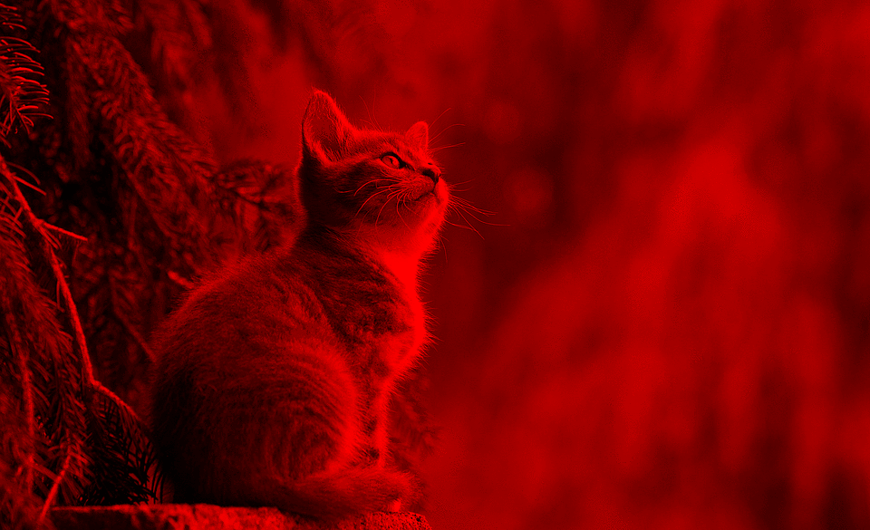
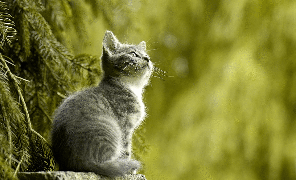
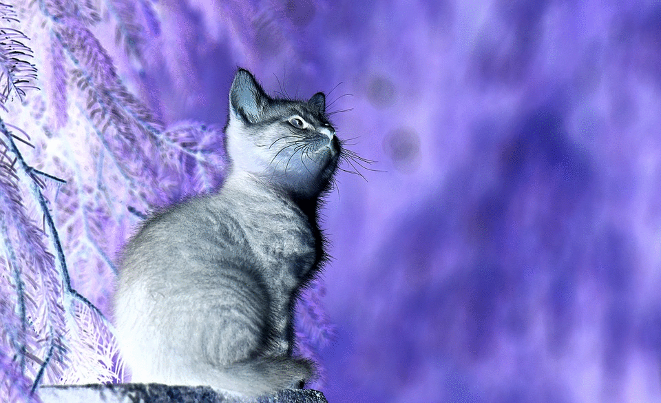
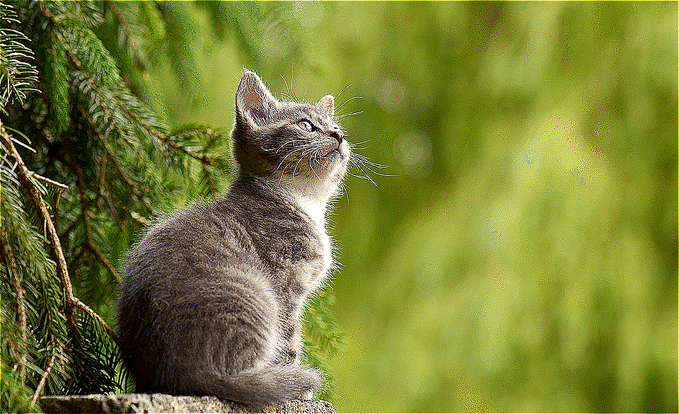
You may also find the following cat picture helpful for testing purposes.

Problem 1: Simple Transformations

Write and document the following three functions

• onlyRed(img). Creates and returns a new image containing only the red aspects of the original image. You can do this by setting all the values in the green and blue values for each pixel to 0.

• deuteranopia(img). Creates and returns a new image that crudely simulates what a red–green colorblind (“deuteranopic”) viewer would see when looking at the image. To do so, set both the red and green pixel values to be the average of the original red and green pixel values. That way the pixels [128, 0, 0] and [0, 128, 0] both come out as [64, 64, 0].

• negate(img). Creates and returns a new image that is a conversion of the original image to its photographic negative form. Modify all colors in a way that turns black into white, white into black, dark colors into light, light into dark, etc. (Don’t worry if you don’t exactly match the color correspondence between a photo negative and its print.)

Finally, write (but do not document) a testing function test_simple(img) that calls the above three functions (separately) on the given image and displays the original along with all three modified versions with appropriately descriptive window titles.

Problem 2: Cropping Images

Write and document a function called crop(img, x, y, width, height) that creates and returns a new image that only contains the pixels contained in the bounding box defined by x, y, width, and height. Here, (x,y) refers to the upper left corner of the bounding box and width and height are its width and height.

Problem 3: Image Convolutions

Introduction

One of the most common ways to apply certain effects to an image is by doing a convolution of the image with a kernel matrix. The kernel matrix encodes a localized transformation that will be applied to every pixel in the image. For example, consider the following 3x3 matrix.

0	-1	0
-1	5	-1
0	-1	0

The above matrix encodes the sharpening transformation and causes pixels to become more distinct from its immediate neighbors. Almost all kernel matrices are an NxN square and have an odd side-length N. (e.g. 3x3 and 5x5). The way an NxN kernel matrix is applied to an image is as follows.

1. To compute the new RGB values of the pixel at location (x,y), you look at the NxN neighborhood of pixels surrounding the point (x,y). In other words, all pixels in the range (x-N//2,y-N//2) to (x+N//2,y+N//2).
2. To compute the R value of (x,y), you iterate over the entire NxN neighborhood surrounding (x,y), multiplying the corresponding matrix value with the R component of the current pixel, and sum up the results.
3. You repeat this process to compute the G and B values of the pixel at (x,y).

This process is visualized in the following animation for the 3x3 sharpening transformation mentioned above. The animation only shows computing one component of each pixel, and the input image is on the left, the kernel matrix is the 3x3 matrix, and the new image produced is on the right.

Notice how the value of each new pixel is computed by multiplying the kernel matrix with the values of the surrounding pixels and taking the sum.

There are many websites that demo the effects of convoluting matrices with images. Check out this website for some examples.

Edge Handling

Since the pixels around the edges of the images do not have a sufficiently large neighborhood, you might notice that in the above animation the pixel values outside the image wrap around to the opposite side of the image. In this assignment, you may implement any edge handling strategy you like, but I recommend that you treat pixels outside the image as black (i.e. [0, 0, 0]). This is a common strategy and is quite simple and will work for our purposes. This may cause a dark border to appear around the output image depending on the choice of kernel matrix.

Implementing Image Convolution

Write (but do not document) a function called image_convolve(img, kernel) that takes an image img and an NxN matrix kernel and creates and returns a new image by convolving it with the kernel.

To do this, you will need to do something like the following:

• Create a new image of the same size.
• Iterate over each pixel of the new image
  • Create sum variables for each component R, G, and B that are initialized to zero
  • Iterate over each cell of the kernel
    • Multiply the R component of the pixel in the neighborhood corresponding to the current kernel cell and add it to the sum for R
    • Do the same for the G and B components
  • After you are finished iterating over the kernel, make sure the R, G, B values are within the range 0..255 and are integers and then create a new pixel using the color_rgb function and insert it into the correct place in the new image

Note that for large images this function takes a while to finish. For example, my sample solution takes approximately 30 seconds to compute a 3x3 matrix on the the cat.gif we were looking at earlier.

Examples

Sharpen

>>> kernel = [[ 0, -1,  0],
              [-1,  5, -1],
              [ 0, -1,  0]]
>>> new_img = image_convolve(img, kernel)
>>> display_image(new_img)

Blur

>>> kernel = [[1/9, 1/9, 1/9],
              [1/9, 1/9, 1/9],
              [1/9, 1/9, 1/9]]
>>> image_convolve(img, kernel)
>>> new_img = image_convolve(img, kernel)
>>> display_image(new_img)

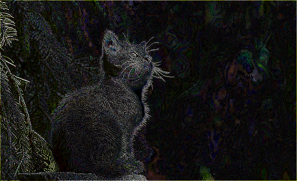
Edge Detection

>>> kernel = [[-1, -1, -1],
              [-1,  8, -1],
              [-1, -1, -1]]
>>> image_convolve(img, kernel)
>>> new_img = image_convolve(img, kernel)
>>> display_image(new_img)

How to Turn in Your Code

a. Make sure that you and your partner are clearly identified at the top of every file you have created for this assignment.

b. All of your files need to be placed into the Hand-in/USERNAME/assignment6 directory. You can do this visually in Finder by copying all of your files in your StuWork/USERNAME/assignment6 directory into your Hand-in/USERNAME/assignment6 directory. (Note that you only need to do this once—it is not necessary for every member of your group to submit separately.)

c. Send all of your files to your partner so they have access to them, too!