The Surface Grower Algorithm

By Steven Clark

Introduction to Surface Grower:

The Surface Grower algorithm is based on work done by David Cohen-Steiner and Frank Da, and is described in their paper "A Greedy Delaunay-Based Surface Reconstruction Algorithm", which can be found here. The description of the Surface Grower algorithm assumes basic familiarity with three-dimensional Delaunay Triangulations; therefore, the next section will introduce them along with other basic computational geometry concepts. If you are already familiar with such ideas, please feel free to skip ahead.

Computational Geometry Primer:

We'll start in two-dimensions. The first observation to make is that three non-co-linear points determine a circumcircle:

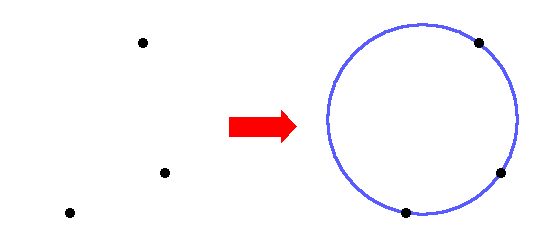
In other words, for any three non-co-linear points, there is a unique circle which passes through all three points. Hopefully this property is fairly intuitive.

It's interesting to note how the size of the circumcircle is affected by the shape of the triangle formed by the three points:

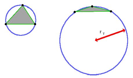
The triangle on the left has both a larger area and a larger perimeter, and yet, it has a smaller circumcircle than the triangle on the right because it is closer to being equilateral.
We're defining r_t to be the radius of the circumcircle of triangle t. This quantity will play an important role in the Surface Grower algorithm, as we will see later.

The concept of the circumcircle helps us define something called the Delaunay Triangulation. The Delaunay Triangulation of a set of points is the set of all triangles having those points as vertices whose circumcircles are empty:

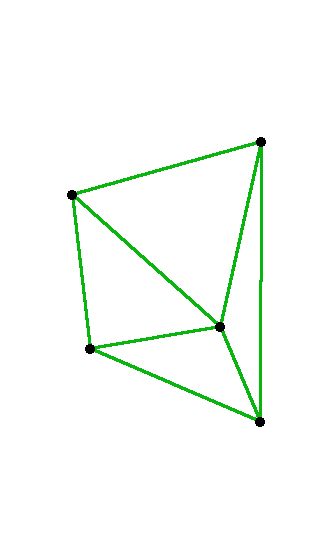
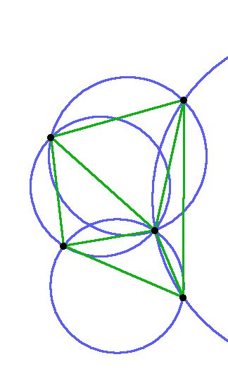
In other words, if you look at the circles defined by the triangles, you can see that they contain no other sample point.

As a brief aside, the Delaunay Triangulation has a geometric dual called the Voronoi Diagram (shown on the right):

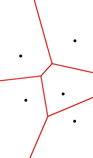
We say that these two are duals, because they are different representations of the same information. One can generate a Voronoi diagram from a Delaunay Triangulation by taking the perpedicular bisectors to each of the Delaunay edges. If two Voronoi cells share a boundary, then they will be connected by an edge in the Delaunay Triangulation. Also, the intersections of the red boundary lines on the Voronoi diagram are the centers of the circumcircles of the triangles. There are many interesting properties which arise from the interactions between Delaunay & Voronoi, but most of them are beyond the scope of this project.

Below is a reconstruction of the Grand Canyon, done using the Bowyer-Watson algorithm--implemented by Ben Anderson in Fall '04.

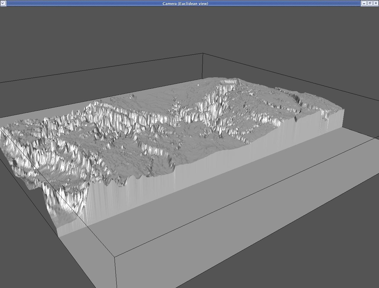
This technique ignores the z-values of the points and performs a simple 2-D delaunay triangulation to obtain the mesh. This algorithm is ideal for topographical data, but doesn't work for a surface which crosses back under itself.

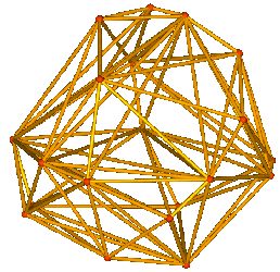
Now we're bumping up to three dimensions. Just like three points define a circle, we find that four non-co-planar points define a sphere. A Delaunay Triangulation in 3D is the set of all tetrahedra having those points as vertices whose circumspheres are empty. This is an example of what a 3-dimensional Delaunay Triangulation might look like:

Here is a depiction of some of the terminology we are going to be using:

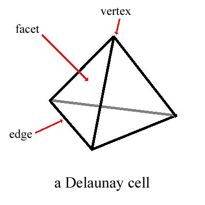
Each tetrahedron will be called a cell. A cell has 4 facets, 6 edges, and 4 vertices. We'll be using the terms facet and triangle somewhat interchangeably.

Surface Grower:

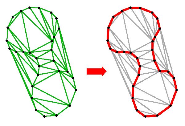
So now you know what a Delaunay Triangulation is. What does this have to do with shape reconstruction? Well, it turns out that a certain subset of the facets formed as a result of a Delaunay Triangulation forms a good approximation to the original surface. A 2D version of the algorithm (curve reconstruction) would hopefully identify the edges in red as the best approximation to the original (admittedly odd) shape:

Therefore, the task of the algorithm could be restated as, "Given a Delaunay Triangulation, identify the collection of facets which best approximates the original surface." Of course, this is easier said than done.

The basic idea behind this algorithm is that we start from a seed facet, and grow the surface outwards from there, adding the most likely facets first in such a way as to keep a continuous boundary. Because we are grabbing the most likely facets first, we say that this is a greedy algorithm.

We will first describe the technique for locating the seed facet, since if you try to start from an incorrect facet (ie one inside the object), you will encounter significant difficulty. Basically, we want to insure that the seed facet is a) actually on the surface, and b) in an area of good sampling density. We do this by finding the facet with the smallest circumcircle. In other words, we iterate through all facets produced by the Delaunay triangulation, and find the one with the smallest r_t.

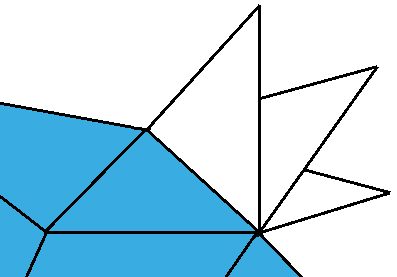
So now that we have the seed facet, we can start growing our surface out from there. At this point, our surface consists of one triangle and three edges. For any given edge on the boundary of the current surface, there are going to be many incident facets:

For each edge, we're going to have to determine which of those facets is going to be our candidate facet. One useful thing to look at is the dihedral angle between the facet you're looking at and the adjoining surface, i.e. the angle between normal vectors 1 and 2:

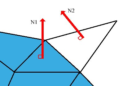
You expect this to be small when the sampling density is good. So the incident facet with the smallest dihedral angle becomes our candidate facet for that edge.

To choose which of the candidate facets to add first, we need a metric with which to compare candidates against each other. We rank them according to their plausibility grade. Two factors go into the plausibility grade, those being the radius of the facet's circumcircle, and the dihedral angle of the facet. The relationship is shown here:
[fix me]
The idea behind the 30 degree threshold is that for sufficiently small dihedrals, the dihedral becomes less of a meaningful metric (especially in the presence of noise), and so we switch over to using the radius to determine the plausibility of the facet.

There are four main data structures we keep track of: The Delaunay Triangulation, a vector of the triangles we have selected thus far, a linked list of Boundary Edges, and a priority queue of candidate facets, sorted by decreasing plausability. At all stages of the algorithm, we have to keep these four up to date and correct.

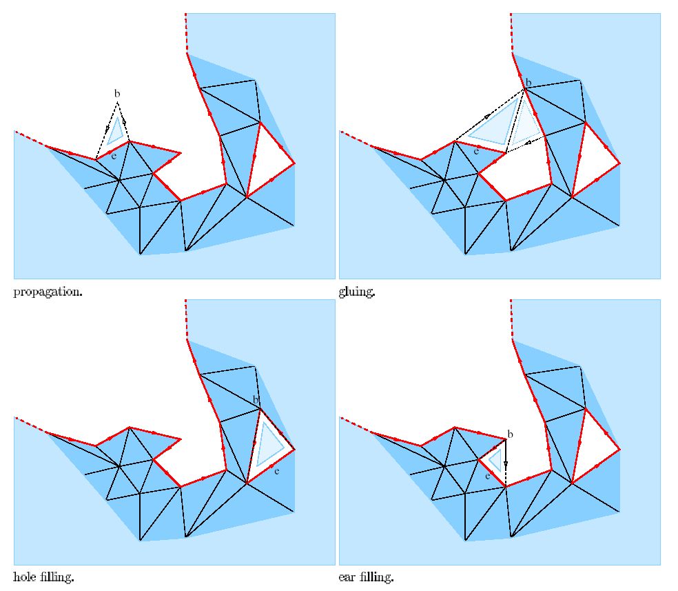
With the priority queue of candidate facets, we can repeatedly pop off the facet with the highest plausibility and attempt to stitch it to the rest of the surface. There are four types of stitching that are allowable, as you can see up here:

Analysis:

The primary strengths of Surface Grower are due to the simplicity of the input requirements; all you need is a list of x, y, z values for points on the surface of the object; this type of data is frequently obtained from a laser-range scanner. Another nice feature is that the input data doesn't have to be constrained to parallel planes: point clouds are ok. And finally, little to no post-processing is required.

The weaknesses of the algorithm are that it is reliant on the feasability of computing a 3D delaunay triangulation. This can be a very computationally expensive task; in our case, we used the open source library CGAL to accomplish this task. Generally, CGAL seemed to be reasonably snappy and robust.

You also are not guaranteed to get a watertight model. Depending on your application, this may or may not matter. And finally, some manual tweaking is required for non-continuous surfaces; essentially, you have to tell it what kind of sampling density to expect.

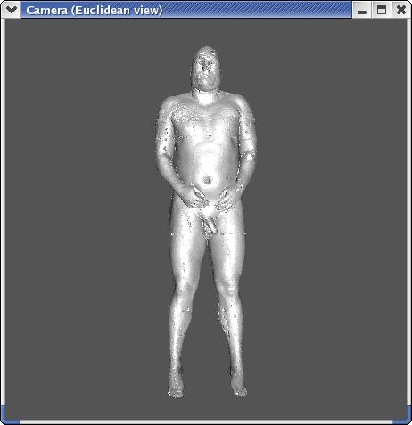
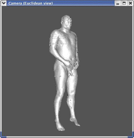
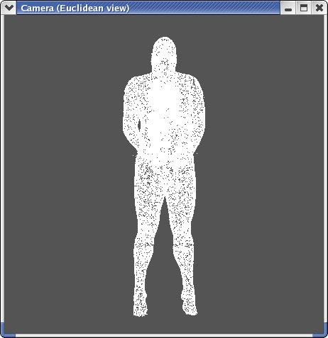
Results:

Input to the algorithm:

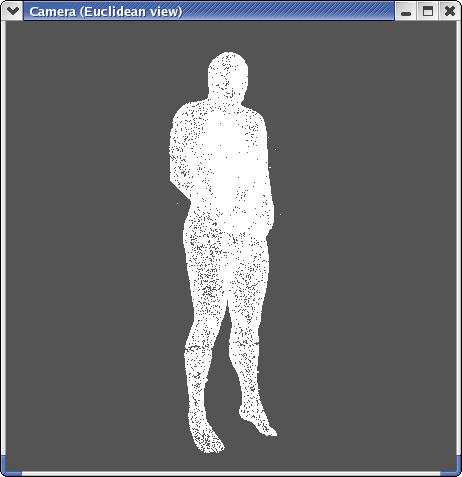
...and triangulated output: